Analysis

Every analysis below runs locally — in a Web Worker in the browser build, and in the same worker inside the desktop app. Nothing is uploaded.

Spectral signatures

Click any pixel to extract its full spectrum. The plot opens below the canvas showing reflectance against wavelength (or band index, when the header carries no wavelengths). Click more pixels to pin additional curves; each gets its own colour and label so you can compare materials side by side.

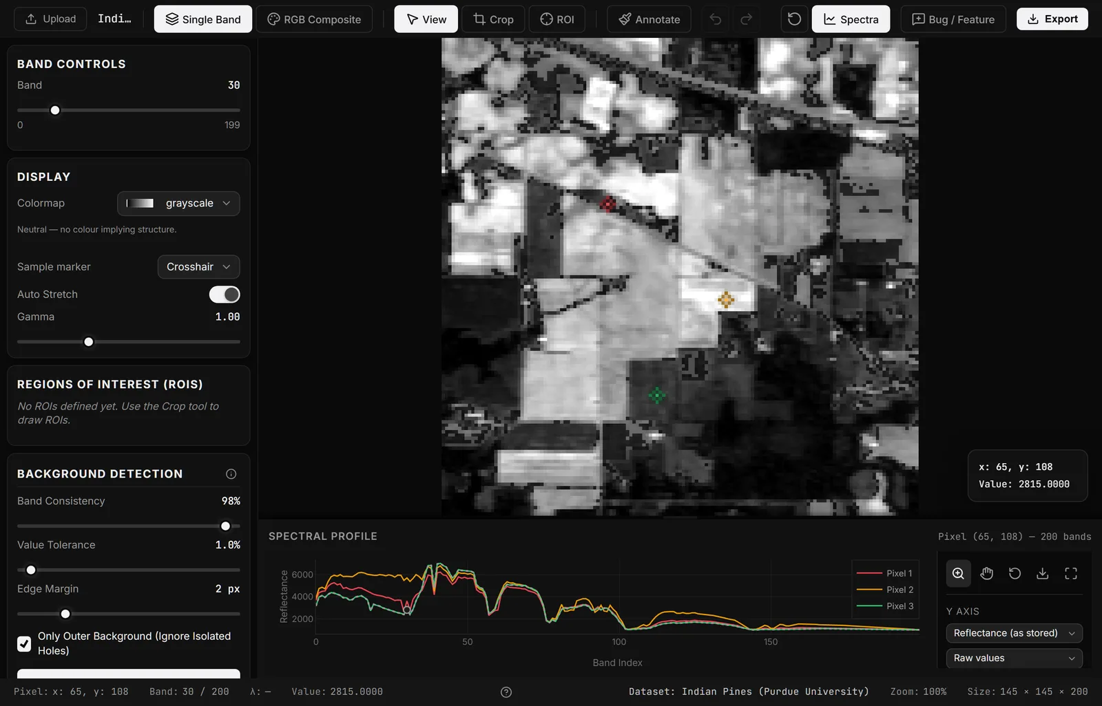
Three pinned spectra from different fields in the scene. The dip near band 100 is water absorption; the step around band 35 is the vegetation red edge.

The plot's axes are configurable:

Control	Options
Y quantity	Reflectance, or Absorbance (`−log₁₀`, computed from reflectance)
Y scale	Raw, Relative (normalised to the maximum), or Percent
X unit	Wavelength (nm) or band index

Absorbance is the convention in chemometrics and NIR spectroscopy; reflectance is the convention in remote sensing. Switching between them is a display transform — the stored data doesn't change.

Class statistics compute the mean spectrum for every annotated class, with its spread, so you can see whether two classes are actually separable before you try to train anything on them.

Spectra can be exported as a vector graphic or as CSV from the plot's export button.

Band Math

Band Math builds a new derived band from two existing ones. Pick band A, band B, and an operation:

Operation	Formula	Typical use
Normalized Difference	`(A − B) / (A + B)`	NDVI, NDRE, NDWI and every other normalised index
Simple Ratio	`A / B`	Band ratios, chlorophyll indices
Difference	`A − B`	Absolute change between wavelengths
Sum	`A + B`	Combining adjacent bands

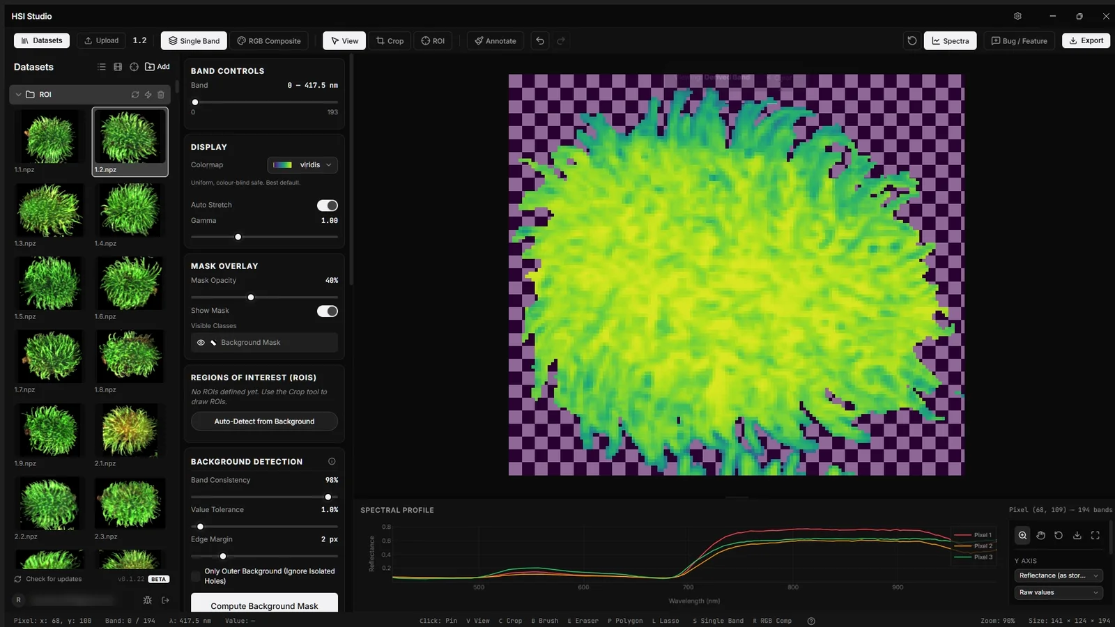
NDVI computed from a 799 nm and a 685 nm band of a rambutan capture, shown in viridis. The index is a new band like any other.

The result becomes a derived band you can view with any colormap, include in an RGB composite, or export. NDVI, for example, is the normalized difference of a NIR band (~850 nm) and a red band (~670 nm).

There are also three RGB composite presets that resolve to the nearest available bands using the cube's wavelength metadata:

Preset	R / G / B target
True Color	650 / 550 / 450 nm
Color Infrared (CIR)	850 / 650 / 550 nm
Agriculture (NDVI-style)	850 / 700 / 650 nm

PCA

Principal Component Analysis reduces hundreds of correlated bands to a handful of components that capture most of the variance. In hyperspectral work it's the standard first move: it denoises, it makes structure visible that no single band shows, and it gives clustering and classification a tractable input.

Choose the number of components and run it. HSI Studio returns:

Each component as a viewable band, with any colormap.
The explained variance per component. This is the number to read — if the first three components hold 98% of the variance, the remaining bands are mostly noise for your purposes.

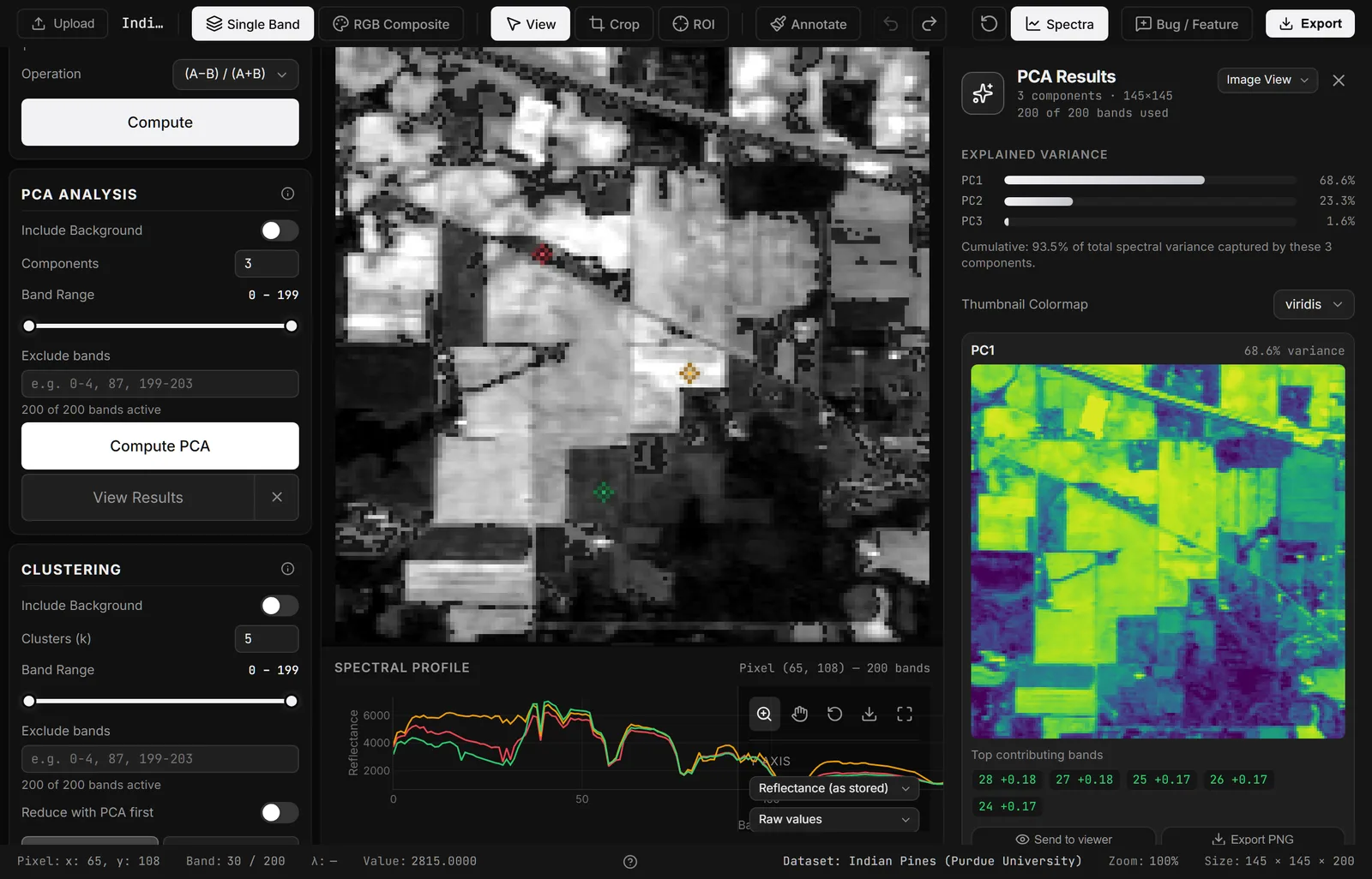
PCA results. Each component is viewable as a band, with the variance each one explains listed alongside.

Component images can be exported directly from the PCA panel.

K-Means clustering

Unsupervised segmentation: pixels are grouped by spectral similarity into k clusters, with no labels required. Useful for a first look at how many distinct materials a scene actually contains.

You can run K-Means on the raw bands or on the top PCA components. Running on PCA components is usually both faster and better — it strips the noise that would otherwise dominate the distance metric. The results panel reports which was used, how many dimensions, and the pixel count per cluster.

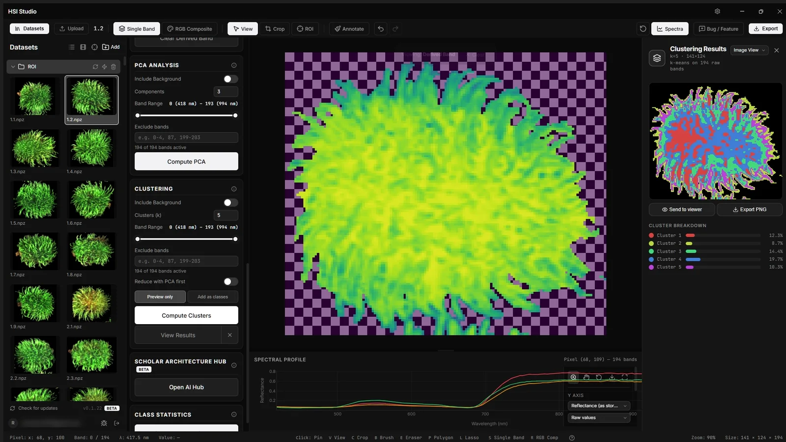
K-Means with k=5 on the same capture. The results panel gives each cluster a colour and reports what share of the pixels it holds.

Cluster assignments can be exported, or promoted into annotation classes as a starting point for supervised labelling.

In-browser classification

Beyond clustering, the browser build can train a supervised classifier on the classes you've annotated, using two classical models:

Random Forest — an ensemble of decision trees. Robust, needs little tuning, handles the high band count without much fuss.
PLS-DA — Partial Least Squares Discriminant Analysis. The workhorse of chemometrics; projects the spectra onto a small number of latent vectors chosen to separate the classes, then classifies in that space.

Both train on annotated pixels and then predict across the whole cube, giving you a classified image and a classification report (per-class precision, recall and support). This runs entirely in the browser and is fast enough to iterate on.

For deep models — 3D-CNNs, transformers, state-space models — and training across a whole dataset rather than a single cube, use the ML Hub in the desktop build.

Auto band removal

Noisy bands — water absorption regions, detector edges — degrade every analysis downstream. Auto Band Removal scores each band's signal-to-noise ratio and drops the ones below a threshold you set. You can preview exactly which bands would be removed before applying, and it's available both interactively and as a batch operation.