ML Hub
Desktop only. Training runs against a local Python interpreter, or on Kaggle. Neither is reachable from a browser tab.
The ML Hub takes a dataset from the Library and trains a model on it. It's organised as a single vertical flow: what to predict → where the labels come from → which model → what compute → run.
Open it from the bottom of the viewer sidebar, under Scholar Architecture Hub — the button reads Open AI Hub.
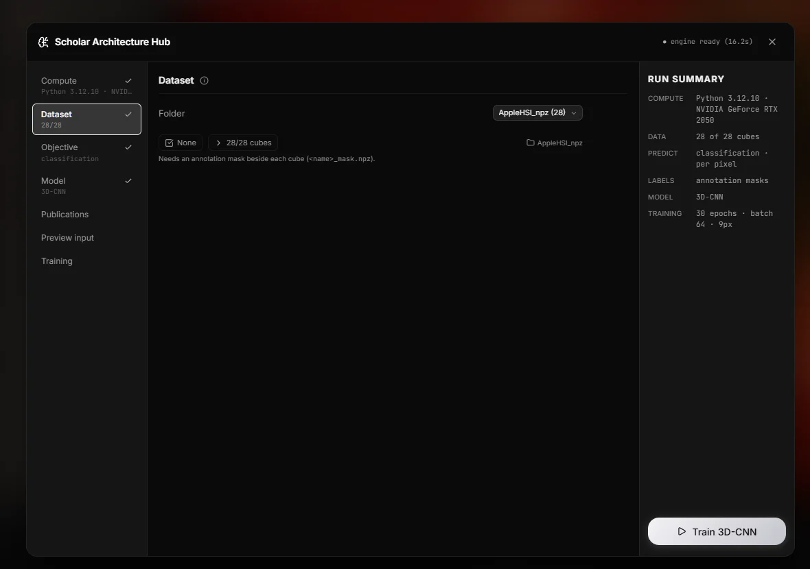
1. Task
Predict — classification (assign a class) or regression (predict a number).
Label level — what one training example is:
| Level | One example is | Typical case |
|---|---|---|
| Each annotated pixel | A spatial window centred on a labelled pixel | Scene segmentation, material maps |
| Each capture | A whole cube | One sample per capture — a specimen, a tablet, a leaf |
Label source — where the ground truth lives:
| Source | How it works |
|---|---|
| Mask | The annotations you painted in the viewer, or a _mask.npz found beside the cube |
| Folder name | The directory a capture sits in is its class. Folder depth is configurable |
| CSV table | A file mapping a key column (filename) to a value column (label) |
| JSON table | The same, in JSON |
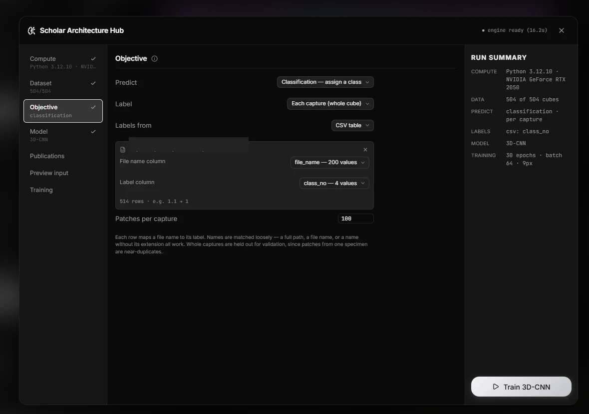
For CSV and JSON you pick the key column, the value column, and the delimiter. HSI Studio inspects the file and shows you what it found, so a mismatch between the table keys and the actual filenames is visible before you start a run rather than after.
For per-capture labelling, patchesPerFile controls how many windows are sampled from each cube — a whole cube is one label but many training examples.
2. Model
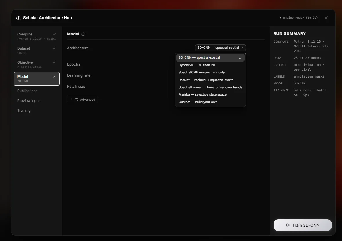
Six built-in architectures, plus a custom builder:
| Architecture | Shape of the idea |
|---|---|
| 3D-CNN | 3-D convolutions over the spatial-spectral volume. The reliable default |
| HybridSN | 3-D convolutions to extract spectral-spatial features, then 2-D convolutions for spatial abstraction. Cheaper than pure 3-D, usually as accurate |
| SpectralCNN | 1-D convolutions over the spectrum only, no spatial context. Fast; the right choice when each pixel is independent |
| ResNet | Residual blocks with squeeze-and-excite channel attention |
| SpectralFormer | A transformer attending across bands, learning which wavelengths matter to each other |
| Mamba | A selective state-space model over the spectral sequence — linear cost in band count |
| Custom | Build a layer stack yourself |
Custom architectures can be assembled in the visual Layer Builder, or written directly as JSON in the spec editor. Starting from a preset — "customise from 3D-CNN" — gives you that architecture's spec as an editable starting point. An architecture diagram renders the layer graph as you build it.
Training hyperparameters:
| Parameter | Default | Notes |
|---|---|---|
| Epochs | 30 | |
| Learning rate | 0.001 | |
| Batch size | 64 | Lower this first if you hit out-of-memory |
| Window size | 9 | The spatial patch around each labelled pixel |
| Validation split | 0.2 | |
| Normalisation | Per cube (min-max) | Or across the whole dataset, or none |
| Max samples per class | 2000 | Caps over-represented classes |
| Class weights | On | Compensates for imbalance in the loss |
Normalisation is the setting people get wrong. Per-cube min-max makes each capture self-consistent and is right when illumination varies between captures. Normalising across the dataset preserves absolute differences between captures — which is what you want when the absolute reflectance level is the signal.
3. Compute
The Hub scans your machine for Python interpreters — everything on PATH, the Windows py launcher, and every conda environment — and reports for each one whether torch and numpy are present, the CUDA version, and which GPUs it can see. Interpreters missing a dependency are listed with what's missing rather than hidden, so you know which environment to install into.
If nothing suitable is found, the Hub says so and tells you what to install (pip install torch numpy). Results are cached; rescan after installing.
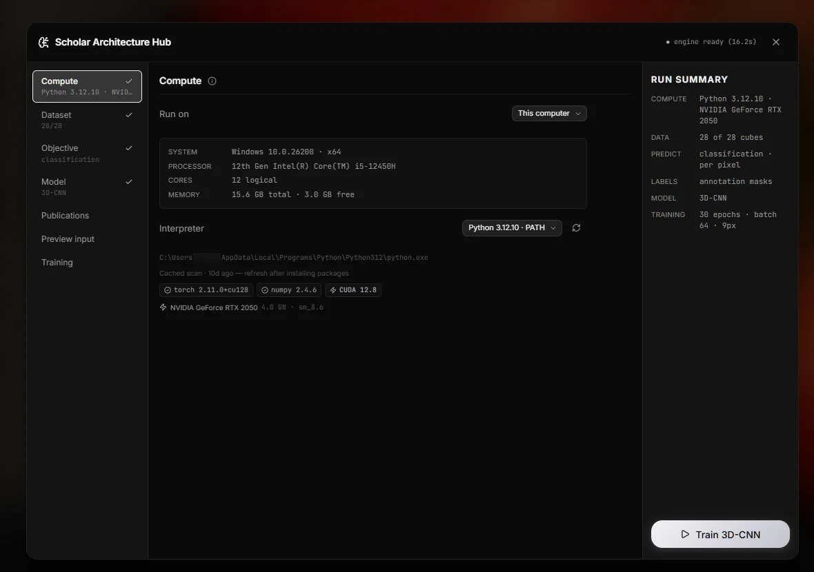
A system readout shows the machine itself — OS, processor, logical cores, memory — separately from the interpreter, because the two are easy to confuse when a run is slow.
When several GPUs are present you pick the device explicitly, so a run doesn't silently take device 0.
Run on offers This computer or Kaggle (cloud). See Kaggle Integration for the remote path.
4. Input preview
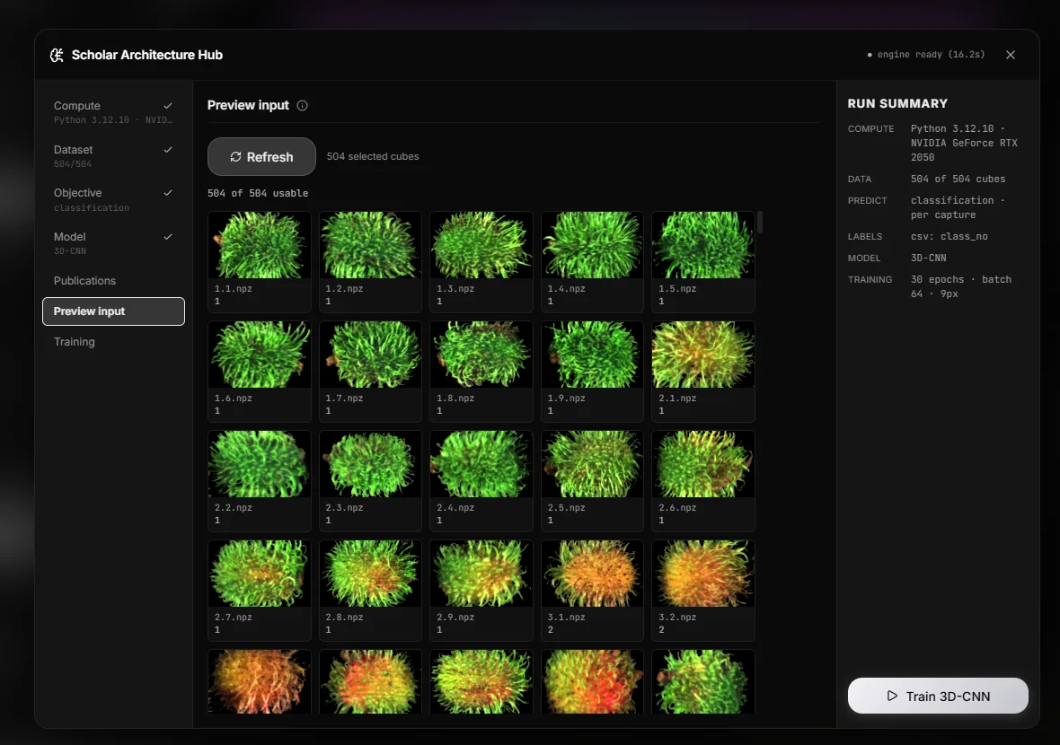
Before running, preview exactly what the model will be fed: the sampled windows, their labels, and the class distribution. This catches the two failure modes that otherwise waste a training run — labels that didn't join to the files, and a class balance so skewed the model will learn the majority class and nothing else.
5. Training
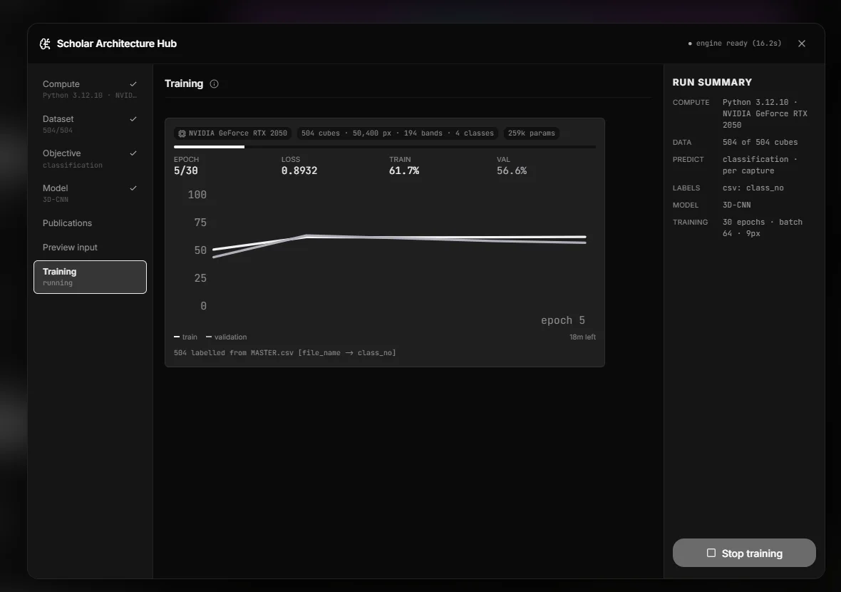
The monitor streams live from the trainer:
- Loss and accuracy per epoch, train and validation, as a chart.
- For regression: RMSE per epoch, plus a predicted-vs-actual scatter — the plot that actually tells you whether a regressor works.
- The raw trainer log, including CUDA out-of-memory diagnostics with the memory figures that caused them.
- Elapsed time and estimated remaining.
Runs can be cancelled. Completed runs produce a checkpoint plus a classification report — per-class precision, recall, F1 and support.
Run history
Every run, local or remote, is recorded. The run list lets you reveal a run's output directory on disk, forget a run, or prune old ones.
Paper search
The Hub includes a literature search over Semantic Scholar, so you can look up the architecture you're about to use without leaving the app. Results carry a citation box with a copyable reference.
Bear in mind that the architecture a paper used on its own dataset is a starting point for yours, not a conclusion about it.
Semantic Scholar works without a key at a low rate limit; you can add your own key in settings for a higher one.