Getting Started
Choose a build
Web — go to hsistudio.online. Nothing to install, no account. This is the full viewer, analysis and annotation suite.
Desktop — download the installer for your platform. The desktop build adds the Dataset Library, batch processing, the ML Hub, and Kaggle integration, and it can read and overwrite files on disk in place rather than working from copies. It requires a sign-in the first time it runs; the licence is then cached locally and re-verified about once a month.
| Platform | Artifacts |
|---|---|
| Windows | hsi-studio-Setup-<version>.exe (installer), hsi-studio-Portable-<version>.exe |
| macOS | hsi-studio-<version>-<arch>.dmg or .zip |
| Linux | hsi-studio-<version>-<arch>.AppImage |
The desktop build updates itself. When a new version is published you'll see an update button in the title bar; on platforms where in-place updates aren't available it opens the download page instead.
Supported input formats
| Format | Extensions | Notes |
|---|---|---|
| ENVI | .hdr + .dat / .raw / .bil / .bip / .bsq | The header and its binary companion must be loaded together |
| NumPy archive | .npz, .npy | Any 3-D array in the archive is treated as the cube |
| MATLAB | .mat | v5 and v7.3 arrays |
| TIFF | .tif, .tiff | Including multi-page / GeoTIFF stacks |
| CSV | .csv | Spectral libraries and pixel tables |
| Images | .png, .jpg | Loaded as 3-band cubes, useful for testing |
| HSI Studio project | .hz | A saved session — cube, mask, classes, ROIs and view state |
On the desktop build these extensions are also registered as file associations, so double-clicking a .hdr, .npz, .mat, .dat or .hz file opens it in HSI Studio directly.
Loading a datacube
Three ways in:
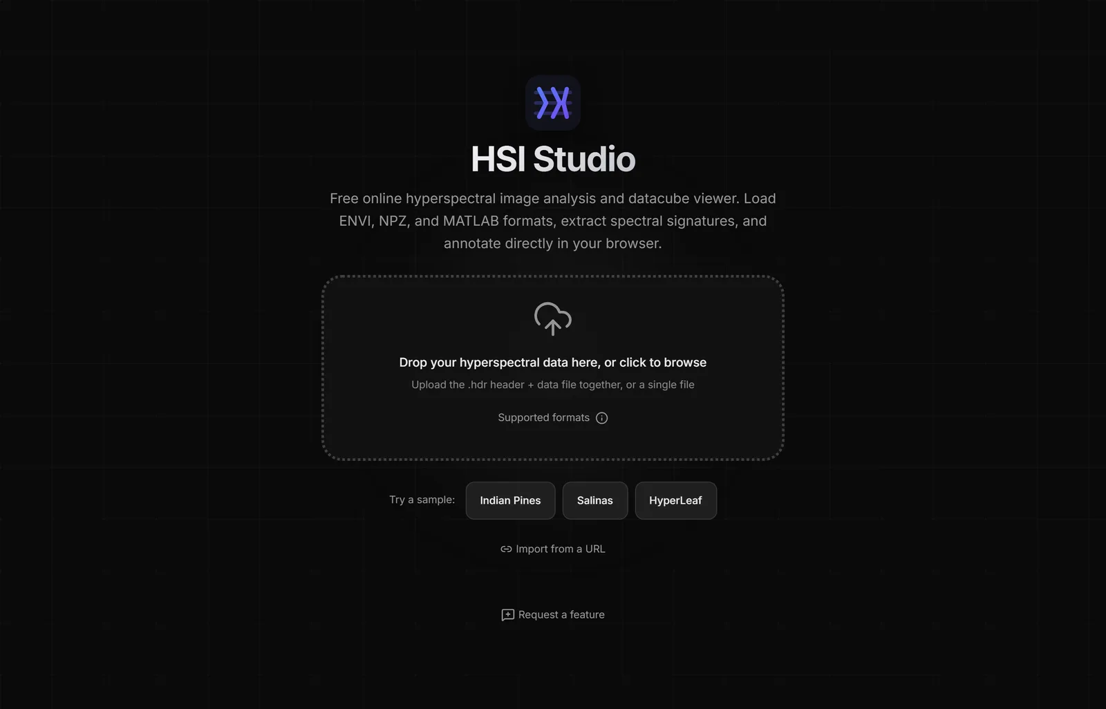
- Drag and drop onto the landing page. For ENVI, drop the
.hdrand its binary companion at the same time — the header alone describes the data but doesn't contain it. - File → Open Datacube (
Ctrl/Cmd+O) on desktop. - A sample dataset from the landing page. Indian Pines, Salinas and Hyperleaf are bundled so you can explore the tool without your own data.
Once a cube is loaded the landing page is replaced by the viewer.
Your first five minutes
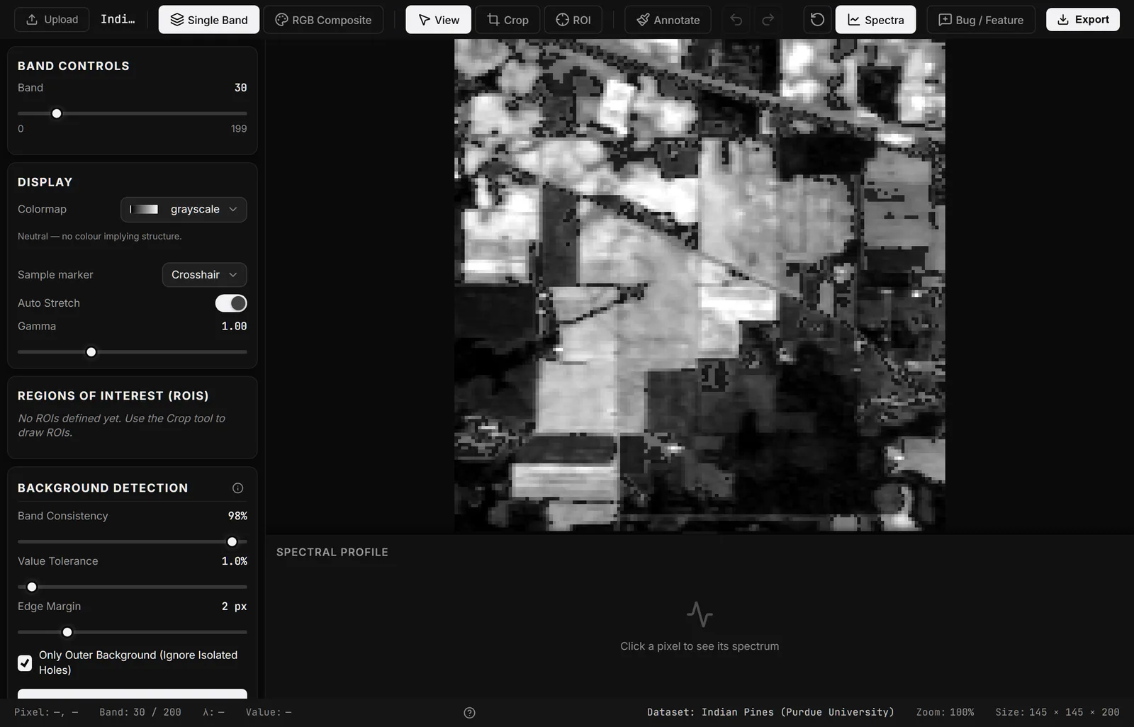
- Scrub the bands. Scroll the mouse wheel over the image, or drag the band slider in the sidebar. Watch how contrast shifts between wavelengths.
- Click a pixel. The spectral plot opens showing that pixel's full reflectance curve across every band. Click more pixels to pin several curves and compare them.
- Switch to RGB. Press
R, or toggle RGB Composite in the top bar. HSI Studio picks bands nearest 650/550/450 nm for true colour when the header carries wavelengths; you can remap any band to any channel. - Paint a class. Press
Bfor the brush and paint over a region, or press the magic wand and click — it selects pixels with a similar spectrum, with an adjustable tolerance. - Export. The Save button in the top right offers the cropped cube, the mask, the current view as a PNG, a pixel-wise CSV, or a
.hzproject you can reopen later.
Where to go next
- Everything the viewer can do: The Viewer
- PCA, clustering and band math: Analysis
- Working with folders of cubes: The Library (desktop)
- Training a model: ML Hub (desktop)